In class the other day I made note of the fact that we sometimes use terms in political science that might have a different meaning as compared to how those same terms are used when we talk about politics in a less technical setting.
Bias
A good example of this is the concept of bias. In more casual settings we typically hear the term bias used as a way of discrediting a source of information. Usually this is because that source is viewed as selectively presenting information, or framing it in such a way, so as to advance a particular political agenda.
In political science when we use the term bias we are often referring to characteristics of a sample or measurement. More specifically, bias is usually used to refer to the gap between the information we have and the “true” underlying value that we’re interested in.
For example, if we’re interested in estimating the average height of a population we might begin by taking a sample of people from that population. Let’s say that we have a population of 1,000 people—then we might sample 100 people from that population and take their average height. We could then use this to estimate the average height of the entire population. Let’s take a look:
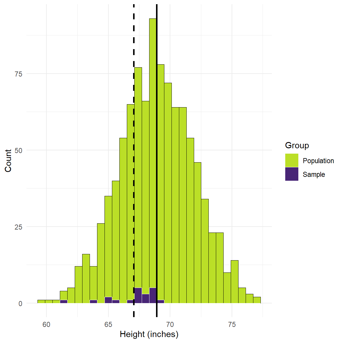
Figure 1: Simulated height values in inches.
Figure 1 shows 1000 simulated height values (in inches). We have a mean of 69 inches and a standard deviation of 3 inches. We’ll set aside whether this is accurate or not for the time being, but it’s close enough for present purposes. The purple values show 20 sample values taken from the population. We’ll also assume for present purposes that our selection process only targets a particularly young portion of the population who are between 12 and 25 years of age, and so many of the people we’ve selected are not fully grown yet. Finally, the dashed line shows the mean height of the sample group and the solid line is the mean value of the population.
A couple of details emerge. First, the size of the sample is necessarily smaller than the population. This is obvious as we only chose 20 out of 1000 people. That’s why we call it a sample! Second, and most importantly for present purposes, you can see that there is a gap between the two mean values—this is the bias in our estimate!
Bias like this can result from a variety of sources. Using height as an example, we might find bias in our sample if the people we sample are all professional basketball players (more likely to be taller), or are all under the age of 25 (younger people are more likely to be shorter). That’s what we did in this example. We could easily do the same thing with another measure like age. If we’re interested in estimating the average age of people in a county or state, and if we only sampled individuals by drawing on people within primary and secondary schools, then our estimate of age would be biased. In this case a biased sample would produce a biased estimate.
No matter what measure you choose to focus on, you have to be cognizant of the potential sources of bias—the things that can lead you to estimate a quantity of interest that is different from the actual underlying value in which you are interested. To be clear, there will almost always be a difference—the question is how close are we to the actual value we’re interested in. Often times these problems can be lessened or even remedied by ensuring that our sample matches the characteristics of the population and/or by collecting more data (i.e. by collecting a larger sample).
In this first example you can see that most of our sampled observations are close to the mean, but this is because this is still where most of the probability mass of the distribution is located. Next, let’s see what happens if we broaden our sampling procedure to ensure we’re sampling from the entire population:
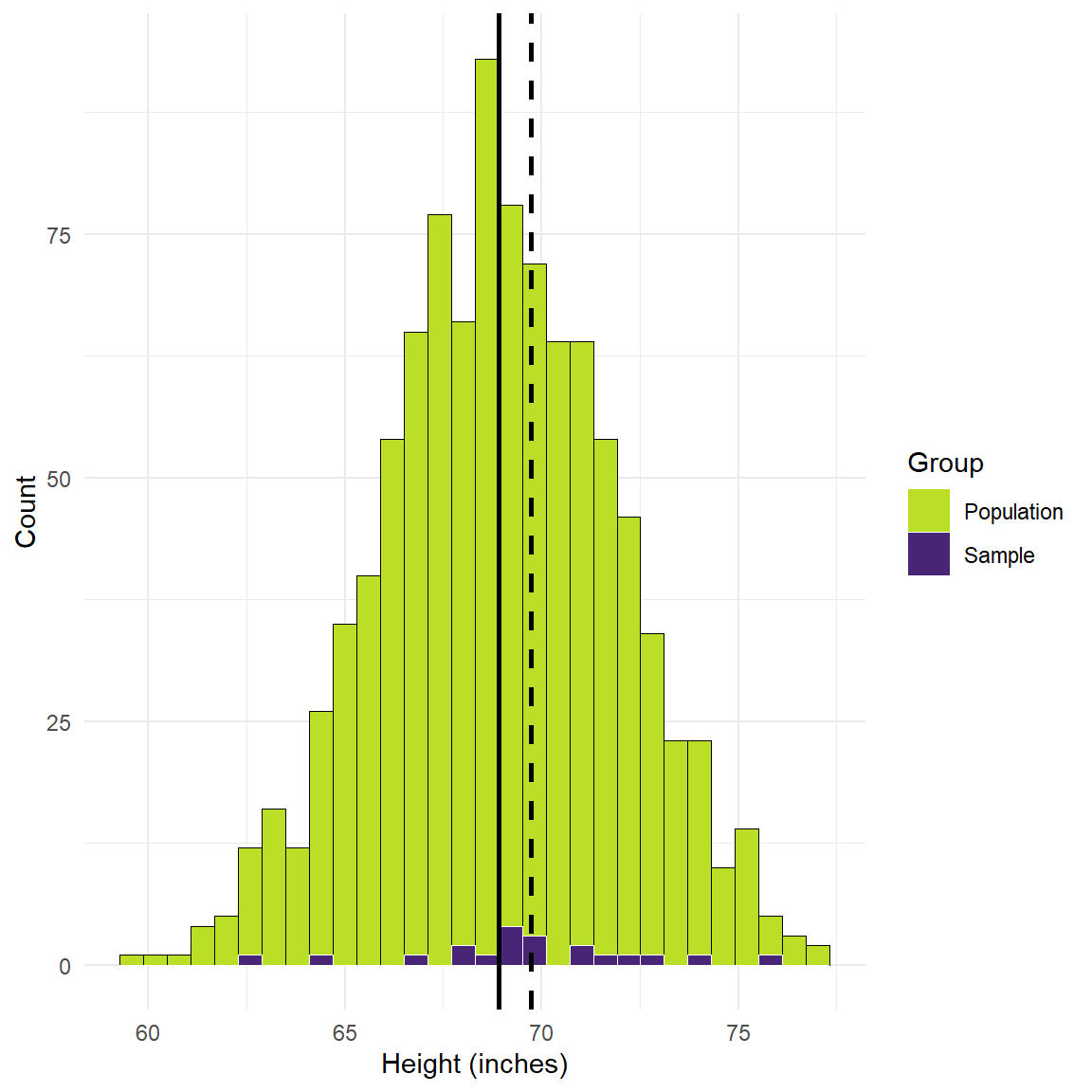
Figure 2: Simulated height values in inches.
There’s still some bias, but the line moves closer to the population mean because we’ve altered our sampling procedure to ensure we’re not just targeting younger people in the population. Now we’re sampling from the entire population. But now our sample mean is above the population mean instead of below. This is a result of the small sample we’ve chosen. Smaller samples are more likely to yield noise. Now let’s see what happens when we keep everything the same but simply increase the size of the sample 10 times:
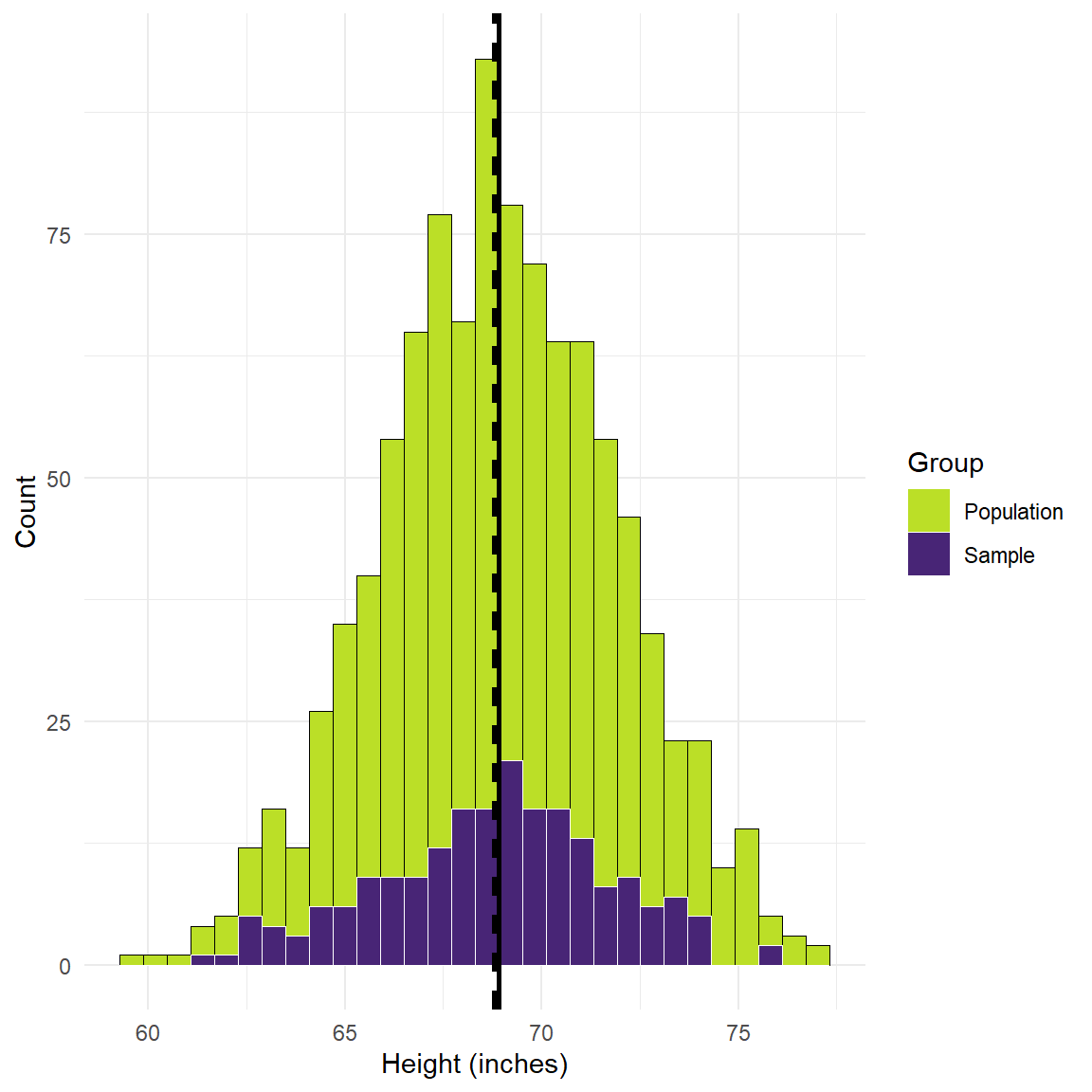
Figure 3: Simulated height values and a sample of 200 individuals
The lines moved closer together, just by increasing the size of the sample! Accordingly, we have reduced the bias of our estimate. Importantly, though, there is still going to be some amount of bias. It is often not something we can ever completely eliminate, but we can try to reduce it.
Accuracy and Validity
Two other terms that we’ll use that have more technical meaning are accuracy and validity. These are maybe less at odds with popular useage than bias, but it’s good to review them just to make sure we’re on the same page.
When we’re collecting data we’re often trying to measure some phenomenon of interest. This is true whether we’re talking about qualitative data collection or quantitative data collection. Validity refers to how close a measure is to the concept that we’re interested in measuring. Reliability refers to how consistent our attempts to measure that concept or phenomenon are.
Figure 3 captures this concept. If we imagine a dart board or a target, validity refers to how close to the bulls eye we get when we try to measure the thing of interest. Similarly, reliability refers to our target grouping. If we’re hitting the bulls eye, or close to it, every time we throw a dart then we’d say that our measurement has a high degree of validity and reliability. If our darts tend to center around the bulls eye but are evenly scattered around the board then then we’d say our measurement instrument is valid, but not very reliable. If our attempts to measure the thing of interest aren’t near the bulls eye and are scattered around, then we’d say our measurement instrument are neither valid nor reliable. ultimately, validity and reliability can both be high, low, or some combination of the two.
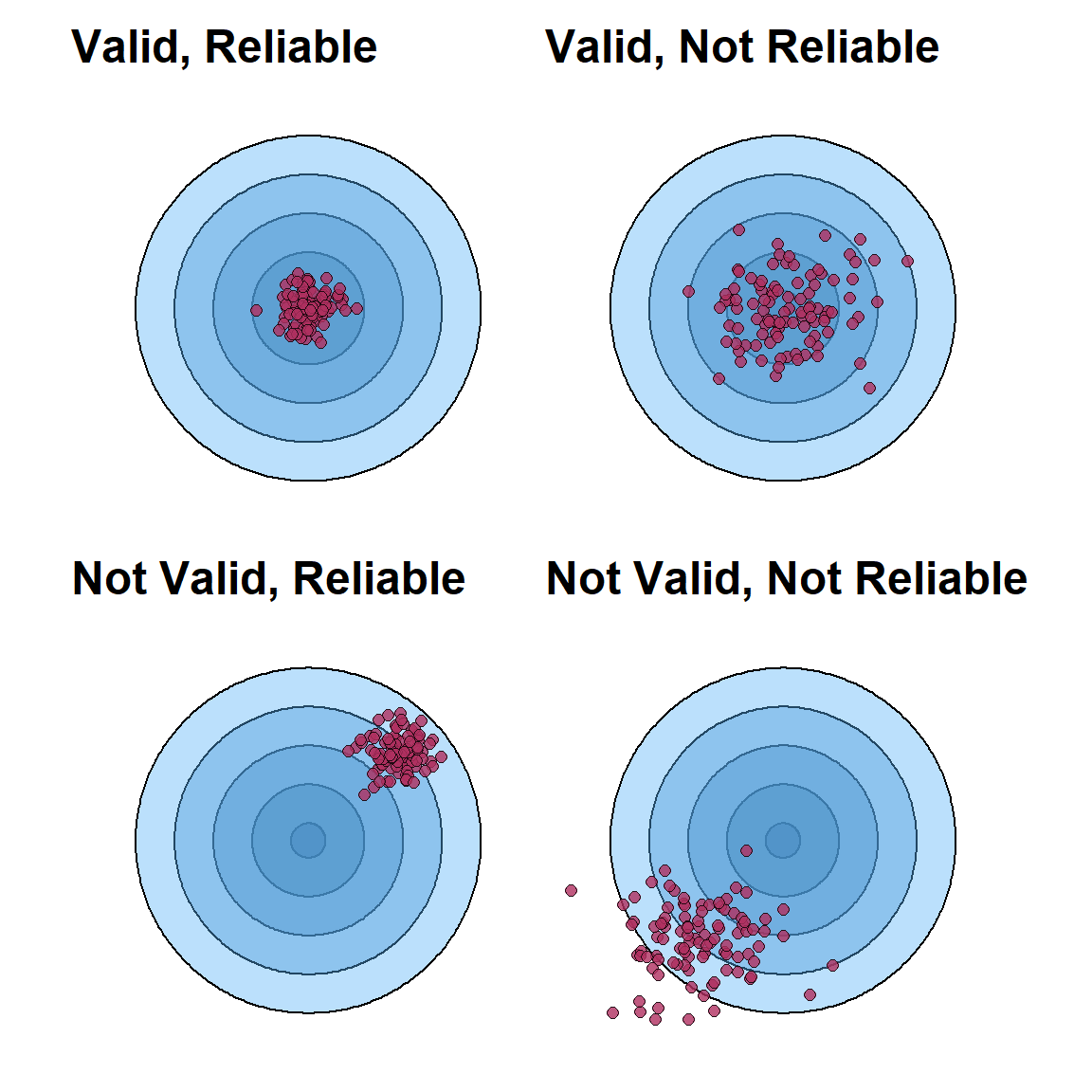
Figure 4: Accuracy and validity
These concepts matter in real life in a wide range of situations. If we want to know how the public feels about a particular policy then the way we phrase a question on a survey instrument can have a huge impact on the quality of the responses with respect to the views we’re trying to tap into. If we have a medical test designed to test for the presence of a particular disease then we want to make sure that the test going to detect that disease with a high rate of success, while also minimizing the chances that it detects other diseases that we’re not interested in.